
Power-Law Learning Curves: Spectral Origins, Schedule Transformations, and Predictive Tests in LLMs
Published:
When power-law responses exist, how training schedules transform them, and whether the resulting mechanism predicts LLM loss
Why should a learning curve follow a power law when every fixed spectral mode decays exponentially?
Power laws are not primitive empirical laws; they are collective dynamical responses. For unresolved target signal and remembered stochastic error, a temporal power law appears precisely when the corresponding cumulative weighted spectrum has matching scale-free mass near zero.
That is the paper’s central result. It separates three questions that are often conflated:
- Existence: when do power-law response components emerge at all?
- Transformation: once they exist, how do learning-rate and batch-size schedules preserve, change, or destroy the power visible in total loss?
- External validity: can the same response coordinates predict controlled LLM learning curves beyond the tractable model?
We give necessary-and-sufficient spectral conditions for the first question and sharp schedule laws for the second. In controlled LLM pretraining, a surrogate fitted on one schedule predicts a held-out schedule without refitting, while matched learning-rate and batch-size implementations nearly collapse in the intrinsic clock.
Two dynamical responses behind a learning curve
In frozen-feature SGD, forcing propagates unresolved target error, while memory measures how much of one stochastic injection remains visible later.
Suppressing finite-width and feedback details, total loss above its irreducible floor has the schematic form
\[L(T)-L_\infty \;\approx\; F(T) +\int_0^T a(u)\,k(T-u)\,\mathrm du.\]The first term is unresolved signal; the integral accumulates the noise-injection history \(a(u)\). Observed loss is therefore a competition between forcing, memory, and past injections.
The spectral if-and-only-if criterion
At first sight, exponential spectral modes and power-law learning curves seem incompatible. The resolution is a moving cutoff.
For a constant schedule, intrinsic time is \(T=\eta t\). At time \(T\), modes with eigenvalue \(\lambda\gg T^{-1}\) have mostly relaxed, while modes with \(\lambda\ll T^{-1}\) remain largely unresolved. Training continuously sweeps this cutoff toward zero. Long-time behavior is controlled not by any single eigenvalue, but by the cumulative weighted spectral mass below \(T^{-1}\).
Two different weights matter:
- target-weighted spectral mass controls forcing;
- squared-spectrum mass controls one-injection memory.
Under the paper’s stability and uniform spectral-window conditions, the main result is
\[\begin{aligned} \nu_W^{\mathcal F}((0,x])\asymp x^{q_{\mathcal F}}\ell_{\mathcal F}(1/x) &\quad\Longleftrightarrow\quad F_{W,>0}(T)\asymp T^{-q_{\mathcal F}}\ell_{\mathcal F}(T),\\ \nu_W^{\mathcal K}((0,x])\asymp x^{q_{\mathcal K}}\ell_{\mathcal K}(1/x) &\quad\Longleftrightarrow\quad \frac{B}{\eta^2}K_W(T)\asymp T^{-q_{\mathcal K}}\ell_{\mathcal K}(T). \end{aligned}\]The equivalence holds separately for forcing and memory. It is an if and only if statement: the low-spectrum weighted mass produces the temporal power, and observing that componentwise temporal power constrains the corresponding low-spectrum mass.
The forward direction explains the emergence of the power law; the converse says that a componentwise temporal power cannot appear without the matching low-spectrum mass law.
Thus a power-law eigenspectrum alone is not sufficient: forcing can decay faster than every inverse power if the target places too little mass in slow directions. Coordinatewise power laws are not necessary either; irregular spectra and targets can produce a clean temporal power through their cumulative mass. Forcing and memory may also have different exponents because they weight the spectrum differently.
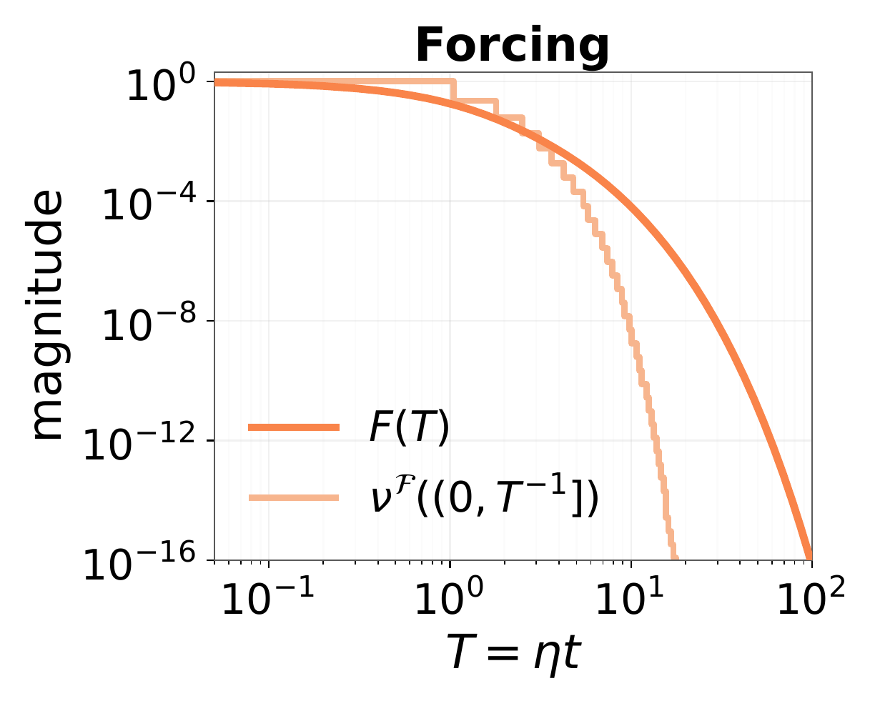
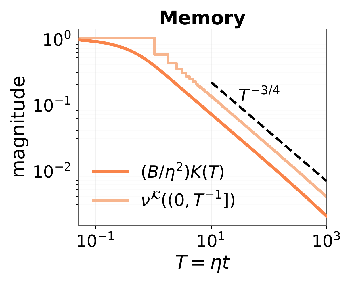
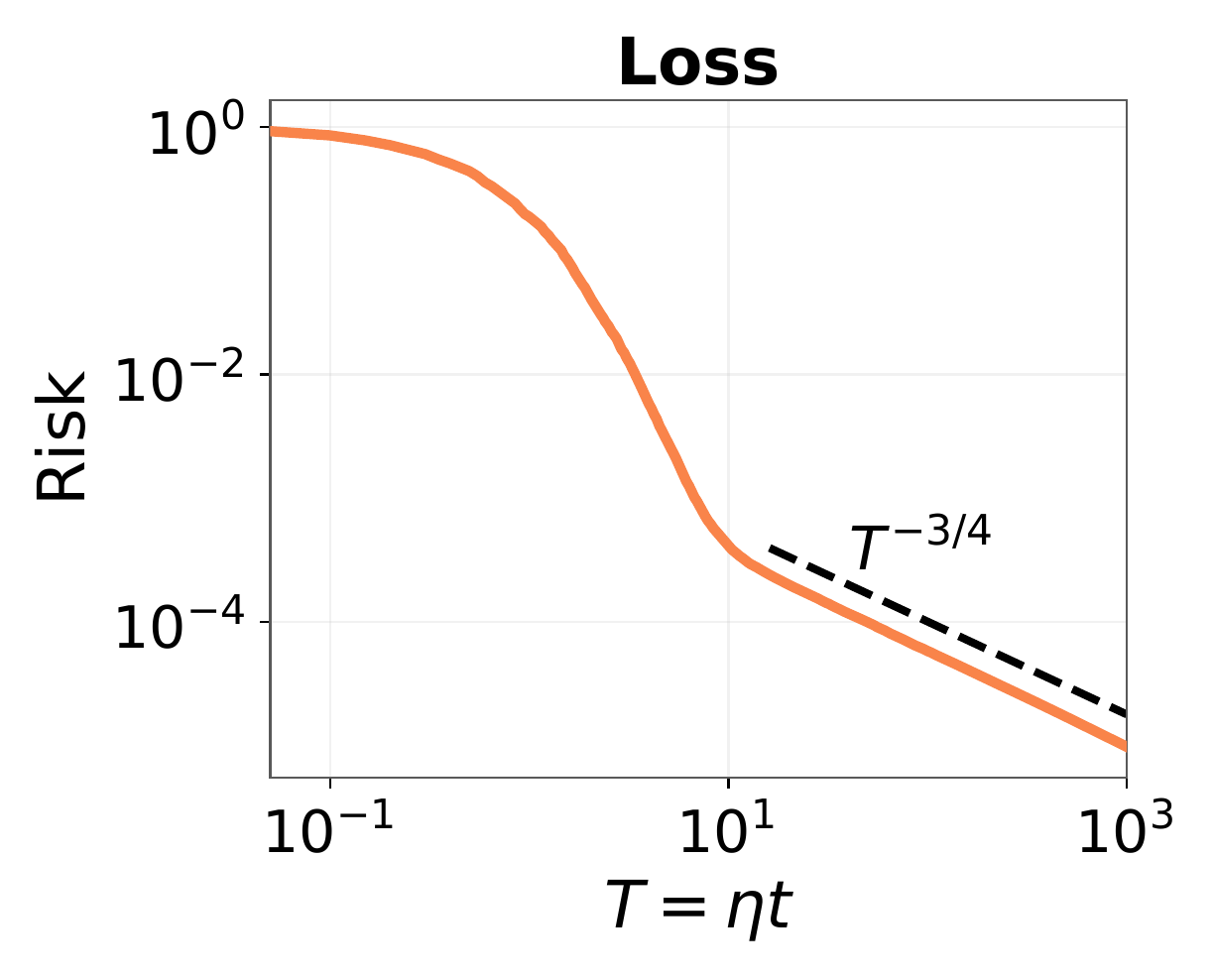
At fixed finite width, decay is eventually exponential. The power law describes an infinite-spectrum limit or a joint width–time scaling window. The theorem is componentwise: it does not by itself characterize total loss.
From component laws to propagation regimes
The response coordinates \((q_{\mathcal F},q_{\mathcal K})\) separate long memory (old injections persist), integrable memory (total memory mass is finite), and finite bulk (width remains coupled to the dynamics). In the power-law random-feature specialization, these become the paper’s \(3+3(+2)\) phase map—a classification of propagation mechanisms, not eight universal total-loss exponents.
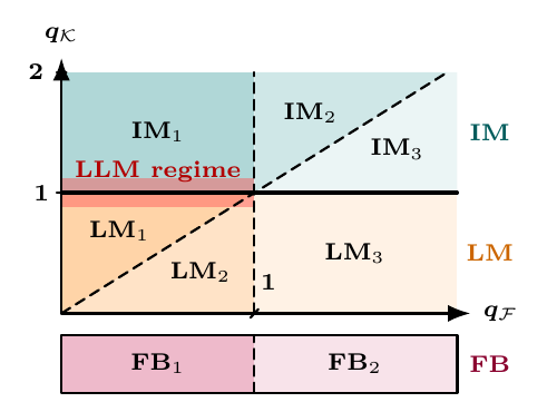
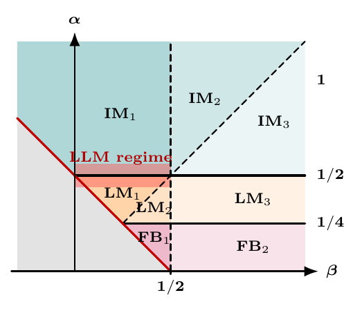
We return below to the LLM fits that locate the red band.
How training schedules transform the response
Once the componentwise power laws exist, plain-SGD learning-rate and batch-size schedules enter through two natural coordinates:
\[T_t=\sum_{s<t}\eta_s, \qquad r_t=\frac{B_t}{\eta_t}.\]Intrinsic time \(T_t\) measures accumulated optimization progress. The ratio path \(r(T)\) controls stochastic-error injection per unit intrinsic time: larger \(B/\eta\) means less injected noise. The full path matters because loss remembers earlier injections. In the response formula above, the leading schedule-dependent scale of \(a(u)\) is \(1/r(u)\).
If memory has tail \(k(v)\sim v^{-q_{\mathcal K}}\) and \(r(T)\sim T^\vartheta\), their convolution gives three outcomes. If \(r\) grows too slowly, fresh noise cannot be forgotten and positive-power decay is destroyed. At intermediate growth, the stochastic gap decays more slowly than clean loss, so the exponent is changed. With sufficiently fast growth, stochastic error becomes subleading and the clean exponent is preserved.
There is also a memory ceiling: reducing late-stage noise cannot erase old injections that are still remembered. Past that ceiling, making \(B/\eta\) grow faster no longer improves the decay exponent.
At the marginal boundary \(q_{\mathcal K}=1\), cumulative memory grows logarithmically, so the pure-power laws acquire logarithmic corrections.
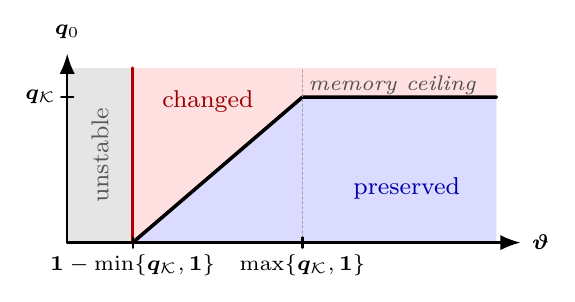
The theory also gives a converse below the long-memory ceiling: the complete noisy–clean gap identifies the ratio path \(B/\eta\), including its slowly varying factor, but cannot identify learning rate and batch size separately. At the ceiling, even this identification is lost.
Testing the response picture in LLM pretraining
The theorems concern frozen random features, not transformers. Our LLM experiments therefore test response-level predictions: whether the coordinates organize end-to-end loss and whether a model fitted on one schedule predicts another.
Test 1: the ratio path affects loss
From one mature 30M checkpoint, eleven plain-SGD tails reached the same intrinsic-time horizon with different \(B/\eta\) growth rates. Faster growth systematically lowered validation loss, with diminishing gains. This one-seed, unequal-compute test shows that the injection path matters, but does not identify an asymptotic exponent or measure the ceiling.
Test 2: two factorizations of the same schedule
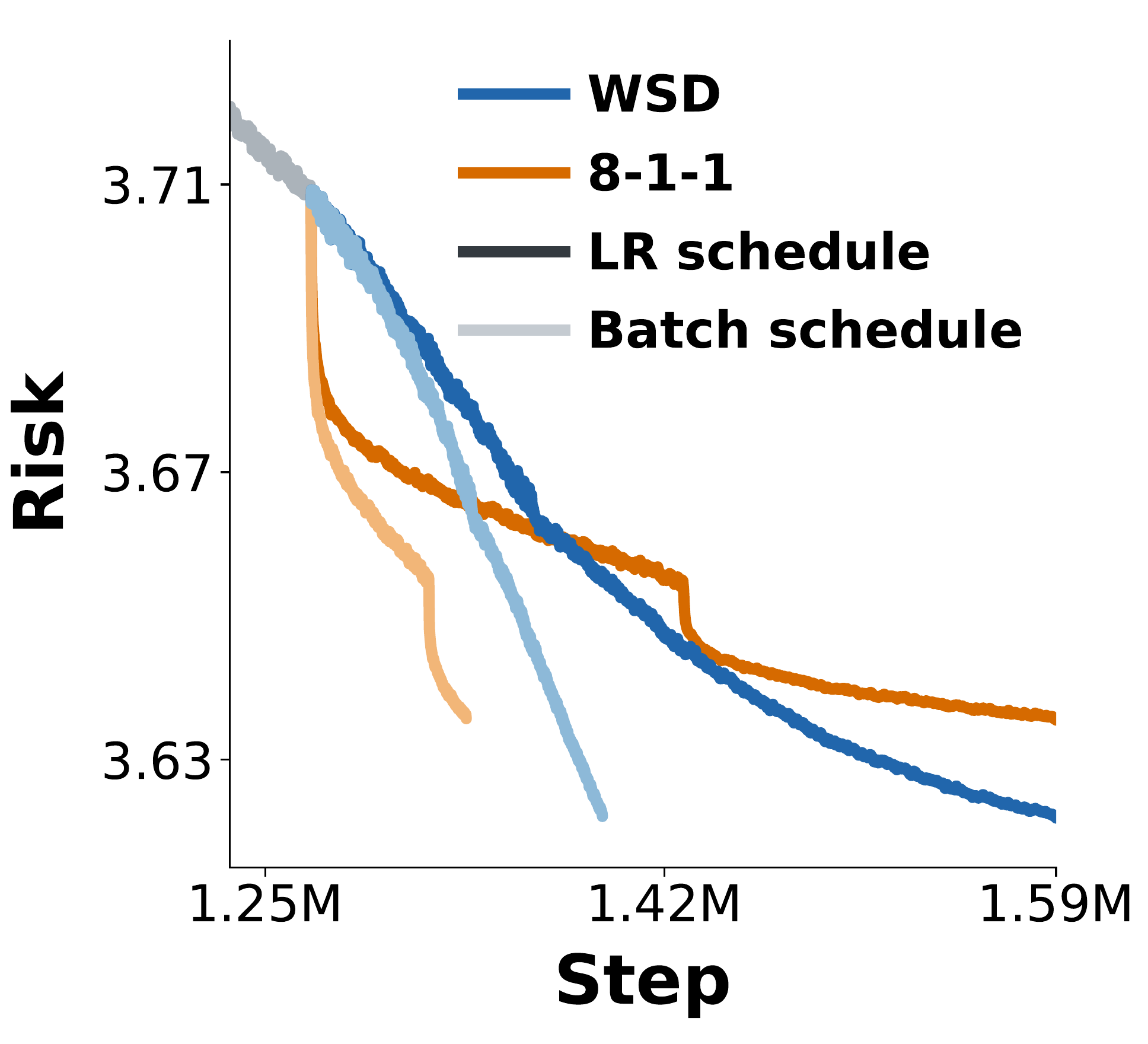
For a 300M nanoGPT trained on 6.5B OpenWebText tokens, a shared 5.2B-token prefix branches into 1.3B-token tails. We implemented both WSD and 8-1-1 ratio paths as either a learning-rate schedule at fixed batch size or a batch-size schedule at fixed learning rate. Each macro step matches intrinsic-time advance, \(B/\eta\), and data. The pairs differ against optimizer step but nearly collapse against intrinsic time.
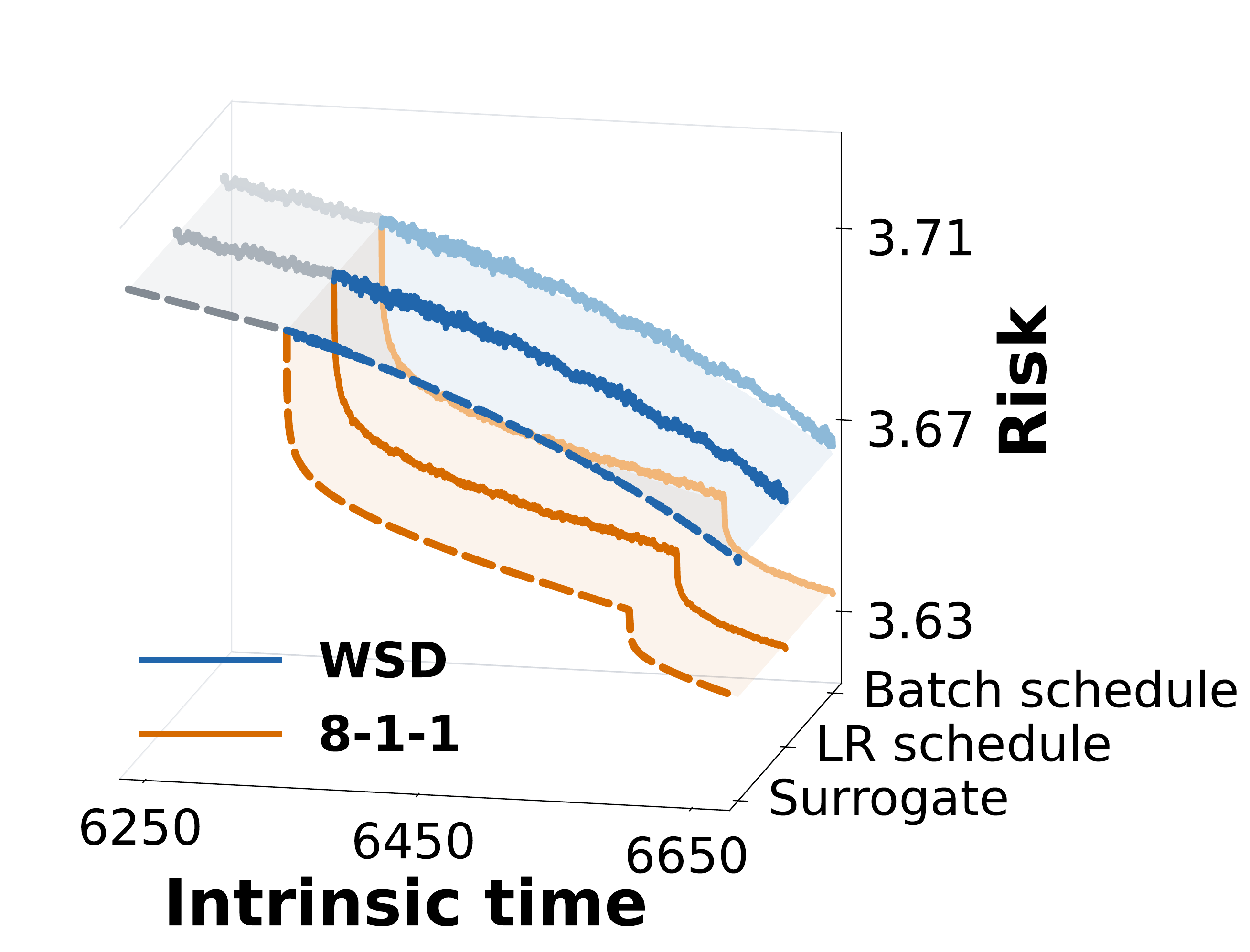
A hybrid-Muon extension shows analogous collapse under empirically calibrated coordinates \(\widetilde T=\sum_t\eta_t^2\) and \(\widetilde r=B/\eta^2\); these are not derived by the plain-SGD theory.
Test 3: fit one schedule, predict another
Approximate collapse is useful, but cross-schedule prediction is a stronger test. We use a seven-parameter finite-window surrogate motivated by the forcing–memory decomposition:
\[\widehat L(T) =L_\infty+A_{\mathcal F}(1+T)^{-q_{\mathcal F}} +\int_0^T \frac{A_0+A_1(1+u)^{-q_{\mathcal F}}}{r(u)} \bigl(1+c_{\mathcal K}(T-u)\bigr)^{-q_{\mathcal K}} \,\mathrm du.\]In the main 300M analysis, we fix \(q_{\mathcal K}=1\) and fit the remaining six parameters only to the raw fixed-batch 8-1-1 trajectory. We then freeze the surrogate and use it to predict the held-out WSD learning-rate trajectory—without refitting.
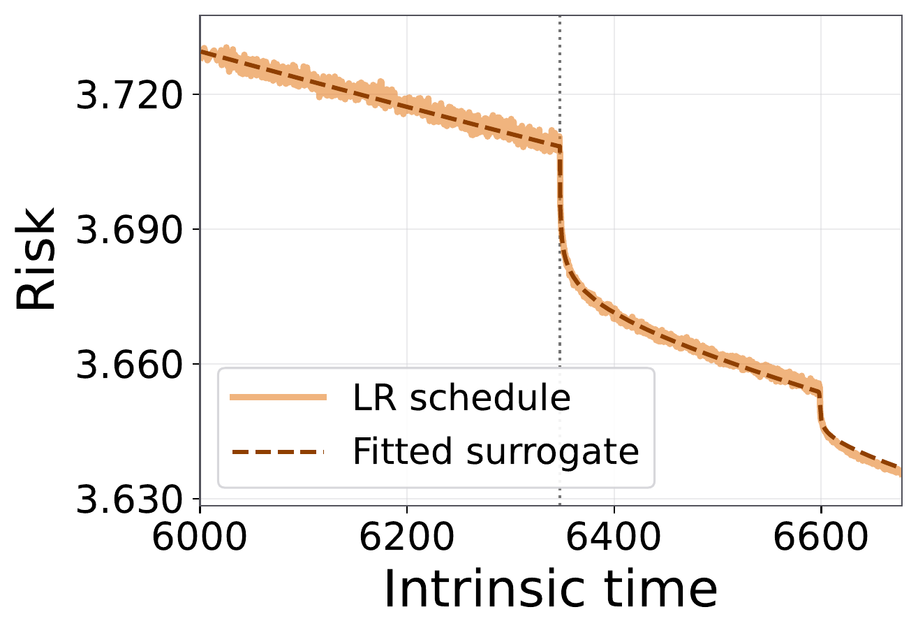
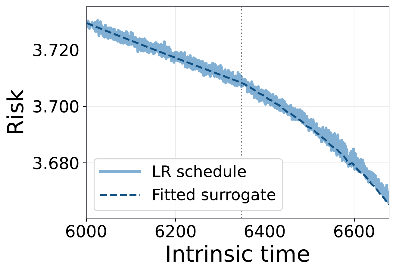
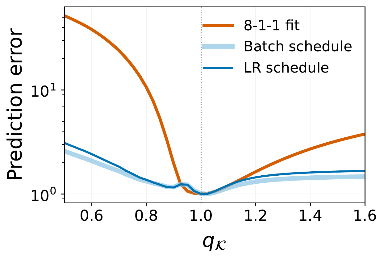
The stronger test is not whether the surrogate fits one curve, but whether parameters inferred from that curve predict what happens after a schedule intervention.
In complementary unrestricted seven-parameter fits across model scales and datasets, we obtain:
| Dataset and setting | Effective \(q_{\mathcal K}\) | Effective \(q_{\mathcal F}\) |
|---|---|---|
| OpenWebText, 124M, 2.5B tokens | 1.017 | 0.374 |
| FineWeb sample-10BT subset, 124M, 2.5B tokens | 0.952 | 0.405 |
| peS2o V2 s2orc full text, 124M, 2.5B tokens | 0.995 | 0.365 |
| OpenWebText, 300M, 6.5B tokens | 0.989 | 0.291 |
Across the tested web and scientific-text corpora, the fitted memory coordinate stays near one while the forcing coordinate remains below one. This places the finite-window response close to the LM/IM boundary. The near-one value is an effective response coordinate: it neither identifies a transformer spectrum nor establishes an asymptotic LLM memory exponent.
What the results change
- A fitted exponent needs a mechanism: ask which response dominates and whether the weighted low spectrum supports a stable power.
- The clock and schedule are part of the observation: report both with the exponent.
- Cross-schedule prediction is stronger than an isolated fit: transfer without refitting tests the mechanism under intervention.
Scope
The theorems concern noisy online SGD with frozen linear random features. The LLM tests do not prove that a transformer has the proxy’s spectrum or an asymptotic random-feature phase. In particular, \(q_{\mathcal K}\approx1\) is an effective finite-window response coordinate. Momentum, AdamW, and representation drift remain outside the theory.
The larger lesson
The main message is not merely that schedules matter. An observed power-law learning curve is the endpoint of a mechanism:
\[\text{weighted low-spectrum geometry} \longrightarrow \text{forcing and memory laws} \longrightarrow \text{schedule-dependent accumulation} \longrightarrow \text{observed loss}.\]Low-spectrum geometry determines whether the componentwise power laws exist. The training schedule determines how those responses appear in total loss. Successful zero-refit prediction in controlled LLM experiments tests whether this description remains useful beyond the tractable proxy.
This post describes joint work by Yichen Wang, Fanghui Liu, and Yudong Chen.