When Do Learning Curves Follow Power Laws?
Published:
During language-model training, loss can follow a power law over a long stretch of a run. A fit to the curve so far gives us a way to estimate how much further the loss might fall if we keep training. This makes learning curves useful well before training is finished.
Extending the fitted curve is straightforward. Knowing when to trust it is harder. The power-law pattern may not last, and even with the same model and data, changing the learning rate or batch size can change the exponent. A curve that looked like a property of the learning task turns out to depend on how we train as well. To predict what happens next, we need to understand where that dependence comes from.
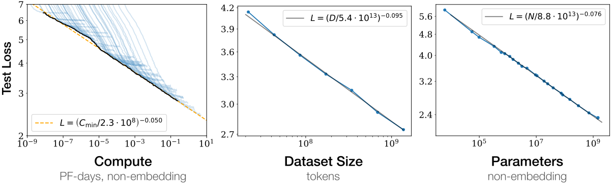
At a fixed compute budget, a larger model leaves fewer tokens for training. Chinchilla captures this trade-off by fitting the final loss of a model with \(N\) parameters trained on \(D\) tokens:
\[L(N,D)\approx L_\infty+\frac{A_N}{N^\alpha}+\frac{A_D}{D^\beta}.\]Here \(L_\infty\) is the fitted loss floor; the other terms describe extra loss from finite model size and training tokens, with fitted amplitudes \(A_N,A_D\) and exponents \(\alpha,\beta\).
For dense Transformers, training compute is approximately \(C\approx6ND\). Choosing the model size and token count that minimize the fitted loss at each budget traces a compute-optimal frontier.
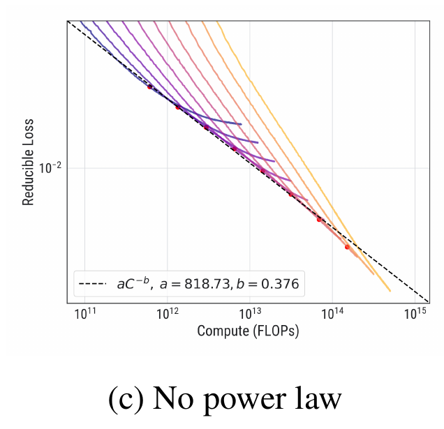
These regularities make power laws useful for planning larger training runs. But the power-law form is not guaranteed across tasks and training recipes.
In Qiu et al.’s synthetic regression experiment, MLPs learning a target with an exponential frequency distribution produce a compute–loss frontier that is not well described by a power law.
The training recipe matters too. In Porian et al.’s language-model experiments, a power law with a fitted loss floor extrapolates well under a tuned recipe, but poorly under other recipes.
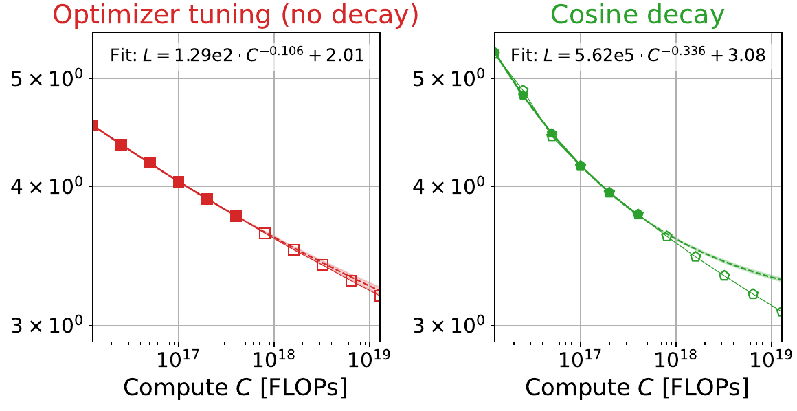
The influence of training is also visible within a single model, not just in the frontier across models. Even with the model and data held fixed, changing the learning-rate schedule can change the fitted power-law exponent of loss versus training steps.
Over a particular training phase, its raw training loss can be fitted as
\[L_{\mathrm{train}}(t)\approx a\,t^{-p},\]where \(t\) counts training steps, \(a\) is the fitted amplitude, and \(p\) is the phase’s decay exponent. To see how training affects \(p\), compare runs with different learning-rate schedules.
Mircea et al. compared separate runs with the same architecture, data, and other settings: one used warmup followed by a constant learning rate; the other used warmup followed by cosine decay.
Compare the 144M model across the two panels: cosine decay raises its fitted late-training exponent from 0.023 to 0.036. The fitted slope depends on the training schedule, not just the model and dataset.
A shared mechanism must explain both why power laws arise and how data and task structure interact with training. A useful test is to fit a response under one schedule and predict another without refitting. For stochastic gradient descent (SGD), we can start with individual updates: each changes the parameters, and its effects can persist through later updates, leaving a history in the loss.
Why SGD has memory
That history is stored in the parameters, but a loss value hides most of it. Two runs with the same current loss can respond differently to the next update. Describing training through loss alone therefore requires accounting for its history.
For a model \(f_\theta\) with training objective \(\mathcal L\), let \(\eta_t\) be the learning rate, \(B_t\) the batch size, and \(\xi_t\) the batch-gradient error. With fresh i.i.d. examples, SGD takes the form
\[\theta_{t+1} =\theta_t-\eta_t\nabla\mathcal L(\theta_t)-\eta_t\xi_t, \qquad \mathbb E_t[\xi_t]=0, \qquad \operatorname{Cov}_t(\xi_t)=\frac{\Sigma(\theta_t)}{B_t}.\]Here expectations are conditional on the training history, and \(\Sigma\) is the single-example gradient covariance. The parameter perturbation \(-\eta_t\xi_t\) therefore has variance scale \(\eta_t^2/B_t\): a smaller learning rate or a larger batch reduces its size. What matters for a later loss is how subsequent updates propagate that perturbation.
A small-noise expansion lets us add up these effects. Write \(F(n)\) for the noise-free validation loss and \(K(n,s)\) for the response at update \(n\) to noise injected at update \(s\), after removing its variance scale:
\[\mathbb E L_{\mathrm{val}}(\theta_n) \approx \underbrace{F(n)}_{\text{baseline learning}} +\sum_{s<n} \underbrace{\frac{\eta_s^2}{B_s}}_{\text{injected variance scale}} \underbrace{K(n,s)}_{\text{effect on the final loss}}.\]The first term follows full-gradient updates from the same initialization and with the same learning-rate schedule; the sum collects the effects of batch noise. Here \(K(n,s)\) still includes the state-dependent strength of that noise, not just its propagation. This is the starting point of the forcing–memory description.
Nothing in this expression yet makes the response a power law. To understand its shape, we need to know how quickly training removes an error.
Derivation details: from SGD updates to the memory response
Fix a horizon \(n\), an initialization \(\theta_0\), and deterministic schedules \((\eta_t,B_t)\). Let \(\theta_t\in\mathbb R^p\) be the parameters before update \(t\). Each update uses fresh i.i.d. examples from the same data distribution. Assume the smoothness and moment bounds required by the expansions below.
1. The size of the sampling noise. For the model \(f_\theta\) and per-example loss \(\ell(f_\theta;z)\), write \(\mathcal L(\theta)=\mathbb E_z[\ell(f_\theta;z)]\) and \(g(\theta;z)=\nabla_\theta\ell(f_\theta;z)\). At update \(t\), let \(z_{t,i}\) be the \(i\)-th example in the batch. The batch gradient \(\widehat g_t\) and its sampling error \(\xi_t\) are
\[\widehat g_t=\frac1{B_t}\sum_{i=1}^{B_t}g(\theta_t;z_{t,i}), \qquad \xi_t=\widehat g_t-\nabla\mathcal L(\theta_t).\]Let \(\mathbb E_t\) denote expectation conditional on the training history, and \(\mathbb E\) expectation over all batches. Define the single-example gradient covariance \(\Sigma(\theta)=\operatorname{Cov}_z(g(\theta;z))\). Conditional independence of the examples gives
\[\mathbb E_t[\xi_t]=0, \qquad \mathbb E_t[\xi_t\xi_t^{\!\top}] =\frac1{B_t^2}\sum_{i=1}^{B_t}\Sigma(\theta_t) =\frac{\Sigma(\theta_t)}{B_t}.\]The parameter perturbation is \(h_t=-\eta_t\xi_t\), so \(\mathbb E_t\lVert h_t\rVert^2=\eta_t^2\operatorname{Tr}\Sigma(\theta_t)/B_t\). This separates the schedule-dependent variance scale, \(\eta_t^2/B_t\), from the state-dependent gradient covariance.
2. How one perturbation travels through later updates. Define the full-gradient update map \(D_t\) and its reference trajectory \(\bar\theta_t\):
\[D_t(\theta)=\theta-\eta_t\nabla\mathcal L(\theta), \qquad \bar\theta_{t+1}=D_t(\bar\theta_t), \qquad \bar\theta_0=\theta_0.\]Inject \(h_s=-\eta_s\xi_s\) at a single update \(s\), using full-gradient updates otherwise. Let \(\delta_t^{(s)}\) be the displacement from \(\bar\theta_t\). With a locally Lipschitz Hessian, subtracting the two updates and expanding for \(t\ge s+1\) gives
\[\begin{aligned} \delta_{t+1}^{(s)} &=D_t(\bar\theta_t+\delta_t^{(s)})-D_t(\bar\theta_t)\\ &=\left[I-\eta_t\nabla^2\mathcal L(\bar\theta_t)\right]\delta_t^{(s)} +O\!\left(\eta_t\|\delta_t^{(s)}\|^2\right). \end{aligned}\]Starting from \(\delta_{s+1}^{(s)}=-\eta_s\xi_s\) and retaining the linear term gives
\[\delta_n^{(s)}\approx-\eta_s A_{n-1}\cdots A_{s+1}\xi_s, \qquad A_t=I-\eta_t\nabla^2\mathcal L(\bar\theta_t).\]Here \(A_t\) is the update Jacobian along the reference trajectory. The product describes how later updates reshape the original perturbation; the empty product is \(I\).
3. How the perturbation changes the final loss. Let \(L_{\mathrm{val}}\) be the validation loss. Define \(G_{n,s}(\theta)\) as the final validation loss obtained by starting from \(\theta\) at update \(s\) and following the remaining full-gradient updates:
\[G_{n,s}(\theta) =L_{\mathrm{val}}\!\left((D_{n-1}\circ\cdots\circ D_s)(\theta)\right), \qquad G_{n,n}(\theta)=L_{\mathrm{val}}(\theta).\]By construction, \(G_{n,s}=G_{n,s+1}\circ D_s\).
Write \(\Psi=D_{n-1}\circ\cdots\circ D_{s+1}\) for the map from parameters after update \(s\) to final parameters, with coordinates \(\Psi_i\). Then \(G_{n,s+1}=L_{\mathrm{val}}\circ\Psi\), and the second-order chain rule gives
\[\begin{aligned} \nabla^2G_{n,s+1}(\theta) ={}&\left[\frac{\partial\Psi}{\partial\theta}(\theta)\right]^{\!\top} \nabla^2L_{\mathrm{val}}(\Psi(\theta))\,\frac{\partial\Psi}{\partial\theta}(\theta)\\ &+\sum_{i=1}^{p} \partial_i L_{\mathrm{val}}(\Psi(\theta))\,\nabla^2\Psi_i(\theta). \end{aligned}\]At \(\bar\theta_{s+1}\), the remaining updates end at \(\bar\theta_n\), and \(\frac{\partial\Psi}{\partial\theta}\) equals \(A_{n-1}\cdots A_{s+1}\). Substituting gives
\[\begin{aligned} \nabla^2G_{n,s+1}(\bar\theta_{s+1}) ={}&(A_{n-1}\cdots A_{s+1})^{\!\top} \nabla^2L_{\mathrm{val}}(\bar\theta_n) (A_{n-1}\cdots A_{s+1})\\ &+\sum_{i=1}^{p} \partial_i L_{\mathrm{val}}(\bar\theta_n)\,\nabla^2\Psi_i(\bar\theta_{s+1}). \end{aligned}\]The propagation matrices thus enter the curvature of the future loss. The first term measures how loss responds to the spread in final parameters. The second captures the shift in their mean caused by nonlinear updates: a mean-zero perturbation need not remain mean-zero after nonlinear propagation. Both contribute at second order, so both must be retained.
Return to the actual SGD trajectory and define \(\theta_s^+=D_s(\theta_s)\), the state after the full-gradient part of update \(s\). Since \(\theta_{s+1}=\theta_s^+ +h_s\), a conditional Taylor expansion gives
\[\begin{aligned} &\mathbb E_s\!\left[G_{n,s+1}(\theta_s^+ +h_s)-G_{n,s+1}(\theta_s^+)\right]\\ &\quad=\frac12\mathbb E_s\!\left[ h_s^{\!\top}\nabla^2G_{n,s+1}(\theta_s^+)h_s\right] +O\!\left(\eta_s^3\mathbb E_s\|\xi_s\|^3\right)\\ &\quad=\frac{\eta_s^2}{2B_s}\operatorname{Tr}\!\left[ \Sigma(\theta_s)\nabla^2G_{n,s+1}(\theta_s^+) \right] +O\!\left(\eta_s^3\mathbb E_s\|\xi_s\|^3\right). \end{aligned}\]The linear term vanishes because \(\mathbb E_s[h_s]=0\), and the second equality uses \(\mathbb E_s[h_sh_s^{\top}]=\eta_s^2\Sigma(\theta_s)/B_s\). The higher-order remainder is controlled by third derivatives of the future loss along the segment from \(\theta_s^+\) to \(\theta_s^+ +h_s\).
4. Adding the effects of all updates. A telescoping sum cancels the intermediate future-loss values, leaving the difference between the final SGD loss and the noise-free baseline:
\[\begin{aligned} L_{\mathrm{val}}(\theta_n)-G_{n,0}(\theta_0) &=\sum_{s<n}\left[G_{n,s+1}(\theta_{s+1})-G_{n,s}(\theta_s)\right]\\ &=\sum_{s<n}\left[ G_{n,s+1}(\theta_s^+ +h_s)-G_{n,s+1}(\theta_s^+) \right]. \end{aligned}\]Taking expectations, define the noise-free baseline \(F(n)=G_{n,0}(\theta_0)\) and the response coefficient
\[K(n,s) :=\frac12\mathbb E\!\left[ \operatorname{Tr}\!\left( \Sigma(\theta_s)\nabla^2G_{n,s+1}(D_s(\theta_s)) \right)\right].\]Let \(\mathcal E_n\) collect the expected higher-order remainders over all updates. Inserting the expansion from step 3 gives
\[\mathbb E L_{\mathrm{val}}(\theta_n) =F(n) +\sum_{s<n}\frac{\eta_s^2}{B_s}K(n,s) +\mathcal E_n.\]Earlier noise has not been removed from this calculation: \(\theta_s\) already depends on all preceding batches. The average defining \(K(n,s)\) therefore includes how earlier noise changes the state reached at update \(s\).
5. The error left by the approximation. Let \(M_{n,s}\) uniformly bound \(|\nabla^3G_{n,s+1}|\) along the Taylor segments, over the sampled histories under consideration. Then
\[|\mathcal E_n| \le\frac16\sum_{s<n} M_{n,s}\eta_s^3\mathbb E\|\xi_s\|^3.\]Omitting \(\mathcal E_n\) gives the response approximation in the main text. At fixed horizon, scaling the sampling noise by \(\epsilon\) makes the retained contribution quadratic in \(\epsilon\) to leading order, while the remainder is \(O(\epsilon^3)\), under uniform derivative and third-moment bounds.
The calculation tells us what \(K(n,s)\) measures: how noise added at update \(s\) affects loss at update \(n\), including the effects of the states reached during training. Describing that response by a positive power law in the time since the perturbation is a further modeling step. The next sections explain how the spectral model produces such a law and how the LLM experiments test whether it predicts loss under a new schedule.
Different directions learn at different speeds
Training removes errors faster in some directions than others. A model with fixed features and trainable output weights lets us calculate those speeds explicitly, as in Paquette et al.’s analysis of compute-optimal scaling.
Consider \(f_a(x)=a^\top\phi(x)\), with fixed features \(\phi\), trainable weights \(a\), and squared loss. Let \(\rho_{j,t}\) be the parameter error along a Hessian eigenvector with eigenvalue \(\lambda_j\). Under small full-gradient steps,
\[\rho_{j,t}\approx\rho_{j,0}e^{-\lambda_jT_t}, \qquad T_t=\sum_{s<t}\eta_s.\]The clock \(T_t\) is intrinsic time. Large positive eigenvalues mean fast learning; small ones mean persistent errors, with learning time proportional to \(1/\lambda_j\).
Loss adds up weighted squared errors across these directions. A slow direction contributes little if there was almost no error there to begin with. Learning speed and importance to the loss are different things.
For SGD in our Gaussian random-feature model, the expected squared prediction error \(R_t\), measured against the noiseless target, satisfies the exact recursion
\[R_t=F_t+\sum_{s<t}K_{t,s}\bigl(R_s+\sigma^2\bigr).\]Here \(\sigma^2\) is label-noise variance. The grouping has changed: \(F_t\) propagates initial error with a finite-batch sampling correction, so it is not the noise-free baseline \(F(n)\). The kernel \(K_{t,s}\) includes \(\eta_s^2/B_s\), while \(R_s+\sigma^2\) explicitly supplies the error generating new noise. Earlier, \(K(n,s)\) included state-dependent noise strength but left \(\eta_s^2/B_s\) outside. The two formulas share a forcing–memory interpretation, not identical definitions of \(F\) and \(K\).
Derivation details: from squared loss to learning time
1. From squared loss to the gradient. Let \(\phi(x)\) be the fixed feature vector for input \(x\), \(y\) its target, and \(a\) the trainable weights. Define the population squared loss and its Hessian:
\[\mathcal L(a)=\frac12\mathbb E\!\left[(a^\top\phi(x)-y)^2\right], \qquad H=\mathbb E[\phi(x)\phi(x)^\top].\]For a minimizer \(a_\star\), the condition \(\nabla\mathcal L(a_\star)=0\) gives \(\mathbb E[\phi(x)y]=Ha_\star\). Hence
\[\nabla\mathcal L(a) =\mathbb E\!\left[\phi(x)(a^\top\phi(x)-y)\right] =H(a-a_\star).\]The gradient is the remaining parameter error transformed by \(H\). This identity is exact for squared loss with fixed features.
2. From the gradient to error dynamics. First consider full-gradient training, without batch-sampling noise. With learning rate \(\eta_t\) and parameter error \(e_t=a_t-a_\star\), the update becomes
\[\begin{aligned} a_{t+1}&=a_t-\eta_t\nabla\mathcal L(a_t),\\ e_{t+1}&=e_t-\eta_tHe_t=(I-\eta_tH)e_t. \end{aligned}\]Let \((\lambda_j,u_j)\) be an orthonormal eigensystem of the symmetric matrix \(H\), and define \(\rho_{j,t}=u_j^\top e_t\). Projecting the update onto \(u_j\) gives
\[\begin{aligned} \rho_{j,t+1} &=u_j^\top(I-\eta_tH)e_t\\ &=(1-\eta_t\lambda_j)\rho_{j,t}, \qquad Hu_j=\lambda_j u_j. \end{aligned}\]Along direction \(u_j\), the gradient is \(\lambda_j\) times the remaining error. In the small-step regime, one update therefore removes a fraction \(\eta_t\lambda_j\) of that error.
3. From the recurrence to a learning time scale. Iterating from the initial error \(\rho_{j,0}\) gives
\[\rho_{j,t} =\rho_{j,0}\prod_{s<t}(1-\eta_s\lambda_j).\]For \(\eta_s\lambda_j\ll1\), using \(\log(1-x)\approx-x\) yields the intrinsic-time approximation
\[\rho_{j,t}\approx\rho_{j,0}e^{-\lambda_jT_t}, \qquad T_t=\sum_{s<t}\eta_s.\]For \(\lambda_j>0\), let \(T_{\mathrm{learn},j}\) denote the intrinsic time needed to reduce the error magnitude by a fixed factor, and \(t_{\mathrm{learn},j}\) the corresponding number of updates. At constant learning rate \(\eta\),
\[T_{\mathrm{learn},j}\asymp\frac1{\lambda_j}, \qquad t_{\mathrm{learn},j}\asymp\frac1{\eta\lambda_j}.\]Large eigenvalues mean short learning times; small eigenvalues mean persistent errors. At time \(T\), modes with \(\lambda_jT\gg1\) have largely decayed, while those with \(\lambda_jT\ll1\) remain close to their initial values.
4. From directional errors to loss. The excess squared loss is
\[\begin{aligned} \mathcal L(a_t)-\mathcal L(a_\star) &=\frac12e_t^\top He_t =\frac12\sum_j\lambda_j\rho_{j,t}^2\\ &\approx\frac12\sum_j\lambda_j\rho_{j,0}^2e^{-2\lambda_jT_t}. \end{aligned}\]The eigenvalues set the decay speeds, while the initial error in each direction sets its weight in the loss. This is why knowing the eigenvalues alone is not enough: we also need to know which directions matter for the target. Batch sampling adds new errors during SGD; the full-gradient calculation above isolates how existing errors decay.
When do these learning speeds produce a power law?
Suppose the target has almost no component along a direction that is slow to learn. There is then little signal to learn in that direction. But batch sampling can still introduce errors there, and those errors take a long time to disappear.
In the example below, the spectrum follows a power law but the target barely uses its slow directions. Forcing disappears faster than every inverse power, yet SGD loss retains a power-law tail. What remains is the memory of batch noise.
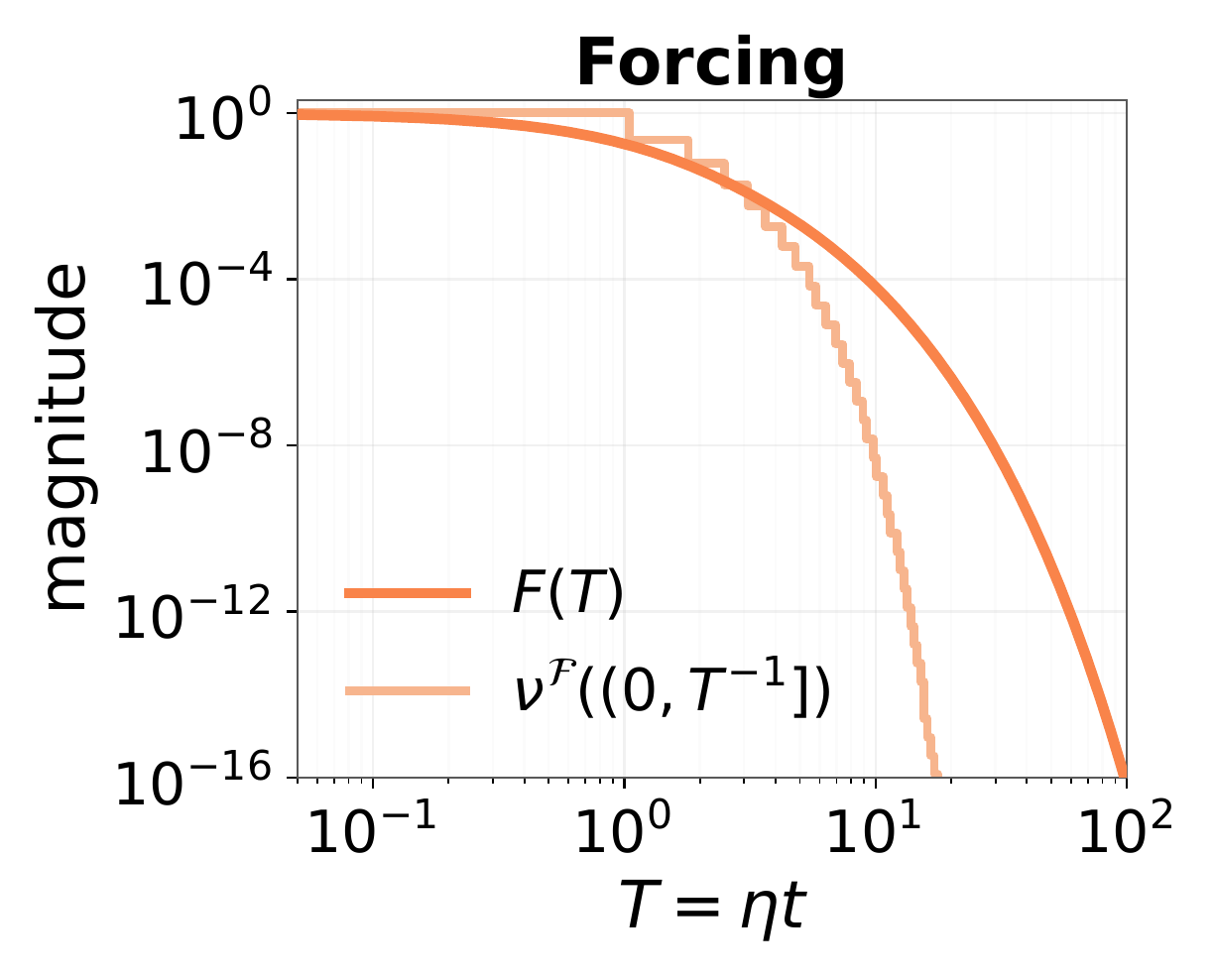
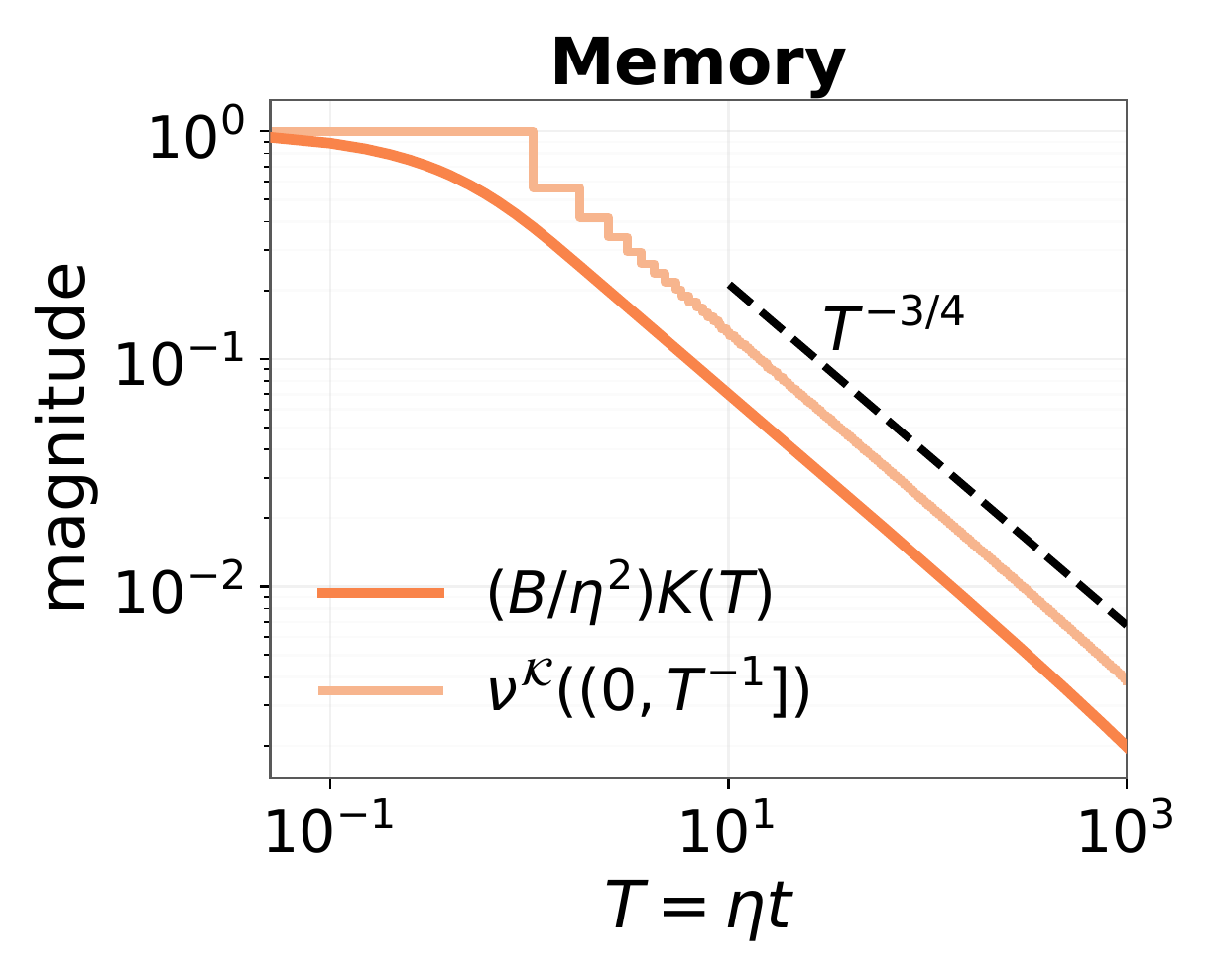
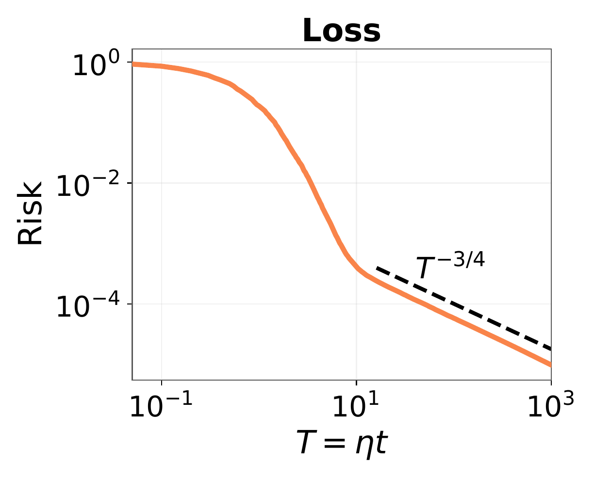
Slow loss decay need not mean slow signal learning. Forcing and memory use the same decay speeds, but assign different weights to them. A fitted loss exponent alone does not tell us which contribution controls the curve.
As training continues, fast directions fade and slower ones take over. At time \(T\), the remaining contribution comes mainly from directions with \(\lambda\lesssim1/T\). We therefore need to add up their weights separately for forcing and memory.
In this model, the fixed features are \(\phi(x)=W^\top x\) and the noiseless target is \(x^\top\theta^\star\), with fixed random-feature matrix \(W\) and target parameter \(\theta^\star\). Let \(\widehat\lambda_j\) and \(\widehat u_j\) be the eigenvalues and unit eigenvectors of \(\Lambda^{1/2}WW^\top\Lambda^{1/2}\), where \(\Lambda\) is the input covariance. Starting from zero output weights, the two cumulative weights are
\[\begin{aligned} \nu_W^{\mathcal F}((0,x]) &=\sum_{0<\widehat\lambda_j\le x} \left|\left\langle\widehat u_j,\Lambda^{1/2}\theta^\star\right\rangle\right|^2,\\ \nu_W^{\mathcal K}((0,x]) &=\sum_{0<\widehat\lambda_j\le x}\widehat\lambda_j^2. \end{aligned}\]If the cumulative weight below \(x\) scales as \(x^q\), then the contribution left at time \(T\) is of order \((1/T)^q=T^{-q}\): training has moved the cutoff down to \(x\sim1/T\). This is how exponential decay along individual directions can add up to a power law.
For a constant schedule, write this random-feature forcing as \(F_W\), its part above the floor as \(F_{W,>0}\), and the delay-dependent kernel as \(K_W\). We express these functions in intrinsic time below. Multiplying \(K_W\) by \(B/\eta^2\) removes its injection scale. The theory also gives the reverse implication: in the large-width, long-time limit, a component’s power-law decay requires the corresponding cumulative spectral weight to have the matching exponent. Schematically,
\[\begin{aligned} \nu_W^{\mathcal F}((0,x])\propto x^{q_{\mathcal F}} &\quad\Longleftrightarrow\quad F_{W,>0}(T)\propto T^{-q_{\mathcal F}},\\ \nu_W^{\mathcal K}((0,x])\propto x^{q_{\mathcal K}} &\quad\Longleftrightarrow\quad \frac{B}{\eta^2}K_W(T)\propto T^{-q_{\mathcal K}}. \end{aligned}\]The positive exponents \(q_{\mathcal F}\) and \(q_{\mathcal K}\) describe forcing and memory separately. Individual eigenvalues need not follow a power law; their weighted totals are what matter.
Three kinds of memory
If every perturbation fades, can we eventually ignore the distant past? The memory curve above follows one injection, but SGD adds noise at every step. Those responses accumulate.
In intrinsic time, write \(k(v)\) for that normalized memory profile after a delay \(v\): for the constant reference schedule, \(k(T)=(B/\eta^2)K_W(T)\). The injection strength is supplied separately. With equally weighted injections, the accumulated response can behave in two ways:
- The responses fade fast enough for their total to approach a finite value. This is integrable memory (IM), with \(q_{\mathcal K}>1\).
- Each response fades, but too slowly for the total to settle. This is long memory (LM), with \(0<q_{\mathcal K}<1\). Cumulative memory keeps growing with the horizon.
At the boundary, \(q_{\mathcal K}=1\), cumulative memory grows logarithmically. No individual perturbation has to be permanent for the total to keep growing.
Finite bulk (FB) needs separate treatment: the response remains tied to model width, rather than a width-independent positive decay exponent.
The finer regions compare how fast forcing and memory decay, and whether the forcing tail has a finite time integral.
The two diagrams connect these behaviors to the learning problem. The left uses response exponents; the right uses a concrete spectrum and target:
\[\lambda_j=j^{-2\alpha}, \qquad |\theta_j^\star|=j^{-\beta}.\]Here \(\lambda_j\) are ordered data-covariance eigenvalues and \(\theta_j^\star\) the corresponding target coefficients. Larger \(\alpha\) steepens the spectrum; larger \(\beta\) reduces target weight in slow directions.
In the LM/IM region with finite target energy, the exponents are
\[q_{\mathcal F}=\frac{2\alpha+2\beta-1}{2\alpha}, \qquad q_{\mathcal K}=2-\frac{1}{2\alpha}.\]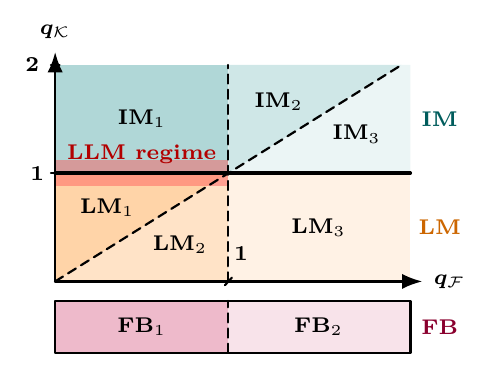
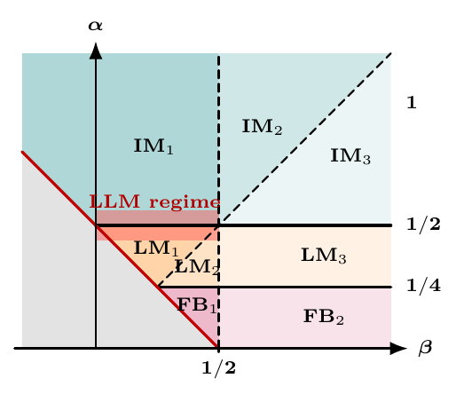
These regions distinguish how forcing and memory propagate, not eight fixed loss exponents. A training schedule changes the strength of successive noise injections. How does their accumulation reshape the observed curve?
How training schedules transform the response
Learning-rate decay often produces a striking change in the training curve: loss that was falling slowly begins to drop much more sharply. In warmup–stable–decay (WSD) training, the learning rate stays constant after warmup until a final decay phase. Follow the gray-green curves in the MiniCPM experiment below: their gradual decline gives way to a sharp drop when decay begins. The same pattern appears at several different stages of training.
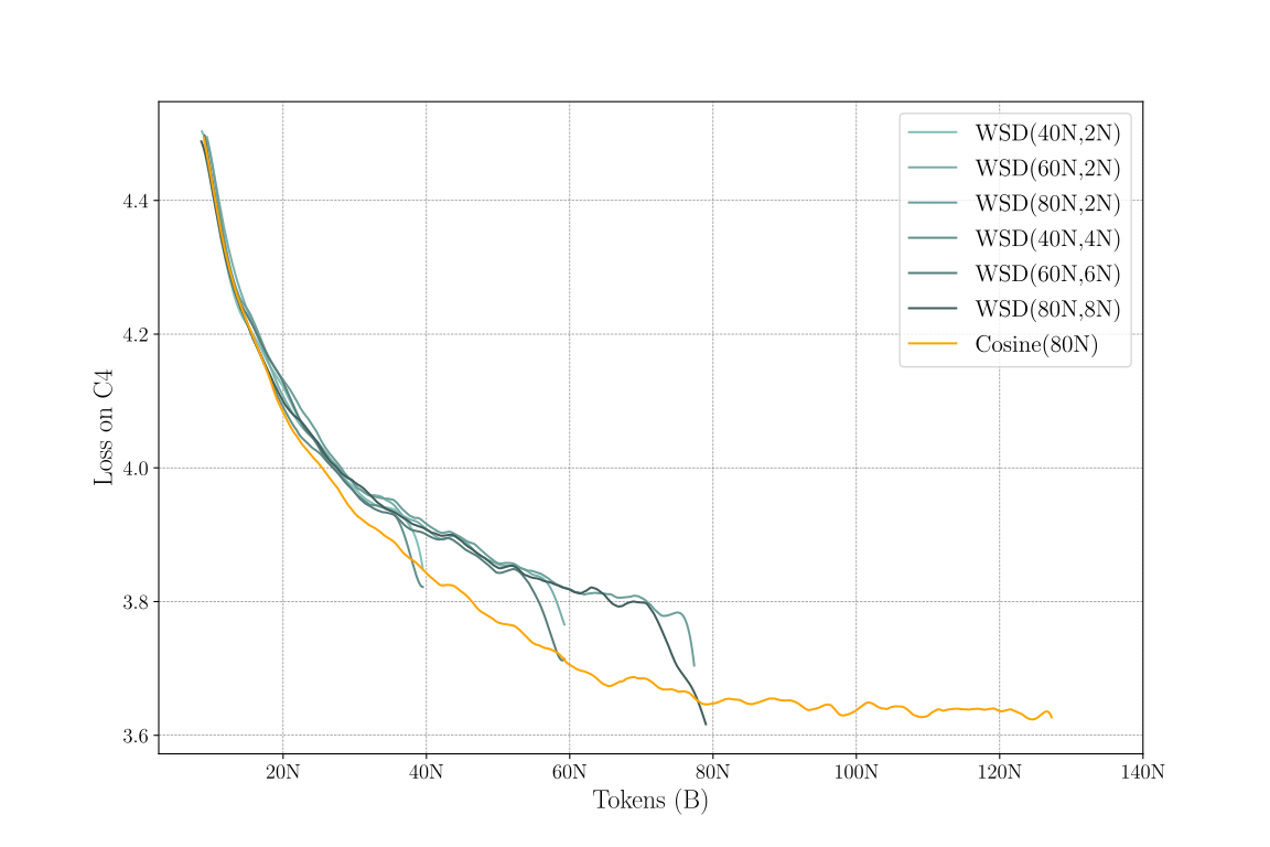
These downward turns make it look as though lowering the learning rate has made the model learn faster. But a faster fall in loss need not mean faster learning of the target: reducing the error caused by stochastic updates also lowers loss. Which effect explains the drop? And if annealing helps, why can’t a more aggressive schedule keep making loss fall faster?
To separate the two effects, start with plain SGD and return to intrinsic time. Lowering the learning rate both shortens the full-gradient update and reduces its noise; increasing batch size reduces noise without shortening that update. The relevant clock and batch-to-learning-rate ratio are
\[T_t=\sum_{s<t}\eta_s, \qquad r_t=\frac{B_t}{\eta_t}.\]An update advances the clock by \(\eta_t\) and injects variance at scale \(\eta_t^2/B_t\). Thus \(1/r_t\) is the noise scale per unit of intrinsic time. Write \(r(T)\) for the ratio along this clock.
This connects increasing batch size with decaying learning rate: both reduce noise per unit of intrinsic time. Since earlier noise can still affect loss, we must match the whole ratio path, not just its final value.
Returning to the power-law random-feature model, the LM and IM scaling law takes the continuum form
\[R(T)\asymp F(T)+ \int_0^T \frac{F(u)+\sigma^2}{r(u)} \,k(T-u)\,\mathrm du.\]Here \(R\) is prediction risk and \(F\) is the random-feature forcing, including its finite-width floor. The exact recursion feeds back \(R_s+\sigma^2\). Under the LM/IM schedule and stability assumptions, accounting for repeated feedback gives the displayed comparison with \(F(u)+\sigma^2\), up to multiplicative constants. It does not set \(R=F\).
Remaining prediction error generates batch noise even with clean labels; label noise adds to it. The ratio \(r(u)\) controls the injection strength per unit of intrinsic time, now outside the normalized kernel \(k(T-u)\), which describes how much of each injection survives until \(T\).
For a concrete example, take an IM regime with \(F(T)\asymp T^{-1/2}\) and \(k(T)\asymp T^{-3/2}\), before the finite-width floor matters. Choose \(r(T)\propto(1+T)^\vartheta\), with its overall scale large enough for stable feedback.
Setting \(\sigma^2=0\) in the integral still leaves batch noise generated by the remaining prediction error. For the three schedules below, this contribution decays faster than forcing, so clean-label SGD has loss of order \(T^{-1/2}\). Its decay exponent is therefore \(q_0=1/2\): here it equals \(q_{\mathcal F}\), but that is not true in general.
Now add the same label-noise variance \(\sigma^2>0\) to each run. In IM, the extra loss relative to clean-label SGD under the same schedule is of order \(T^{-\min\lbrace\vartheta,3/2\rbrace}\). The slower-decaying contribution determines the total loss. Up to constant factors, the three schedules give:
| Ratio growth \(r(T)\) | Extra loss from label noise | Total loss |
|---|---|---|
| \(T^{1/4}\) | \(T^{-1/4}\) | \(T^{-1/4}\) |
| \(T\) | \(T^{-1}\) | \(T^{-1/2}\) |
| \(T^2\) | \(T^{-3/2}\) | \(T^{-1/2}\) |
In the first row, label noise changes the observed exponent; in the second, its effect fades fast enough to preserve the clean exponent. The last row reaches the memory ceiling: increasing \(\vartheta\) further cannot make the extra loss decay faster than the \(T^{-3/2}\) tail left by old injections. The total loss is already limited by forcing at \(T^{-1/2}\).
For power-law memory and ratio growth, comparing this extra loss with the clean loss gives three outcomes:
- Destroy: the extra loss does not decay as a positive power.
- Change: it decays more slowly than the clean loss and sets a new exponent.
- Preserve: it decays at least as fast, leaving the clean exponent unchanged.
The diagram compares the clean excess-loss exponent \(q_0\), describing decay above its floor as \(T^{-q_0}\), with the ratio-growth exponent \(\vartheta\), defined by \(r(T)\sim T^\vartheta\).
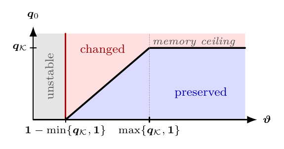
Fix \(q_0\) and move horizontally to the right, increasing \(\vartheta\). If \(q_0<q_{\mathcal K}\), we eventually cross from changed into preserved: the extra loss now decays at least as fast as the clean excess loss. If \(q_0>q_{\mathcal K}\), our horizontal line stays above the memory ceiling, no matter how far right we go. The extra loss has a decay exponent capped at \(q_{\mathcal K}\), so more aggressive suppression cannot recover the clean exponent.
From schedule laws to schedule design
A ceiling on the exponent still leaves a practical choice: with a fixed data budget and ending intrinsic time \(T\), where should we spend extra samples? They help most where the noise they suppress would otherwise persist until the end.
In the LM/IM response model, balancing source strength against this future effect gives the optimal ratio
\[r_T^\star(u) \propto \sqrt{k(T-u)\bigl[F(u)+\sigma^2\bigr]}.\]The data budget fixes the normalization. The square root balances noise generated now against its future effect: some early perturbations will have faded by the end, while others remain influential. Current loss alone does not capture that difference. Bordelon and Mori’s optimal-control analysis offers a complementary route to learning-rate design.
Learning-rate and batch-size schedules can implement the same ratio path. Optimizing training duration and model width then gives phase-dependent data and compute scaling laws. This connects the two scales in the opening: individual learning curves determine what can be achieved by choosing across models.
From theory to LLM pretraining
An LLM keeps changing its representations, unlike the fixed-feature model above. But describing its loss need not require reproducing every change in its parameters.
This leaves room for a broader possibility: forcing–memory may be a coarse-grained response law of SGD, not merely a description of a linear model. Different parameter trajectories could produce similar loss responses. Changing the training schedule lets us test whether that response transfers.
Two implementations of the same ratio path
First, keep the ratio path the same but implement it differently: lower learning rate at fixed batch size in one run, and increase batch size at fixed learning rate in another. Match their clocks and ratio paths.
We did this for a 300M plain-SGD LLM on 6.5B OpenWebText tokens. All runs share the first 80% of the token budget, then branch from the same checkpoint for the remaining 20%. In the fixed-batch runs, WSD lowers the learning rate gradually over that tail, while 8-1-1 uses two lower-rate stages of 10% each. If intrinsic time and the ratio path capture the main schedule dependence, each learning-rate/batch-size pair should follow nearly the same loss curve.
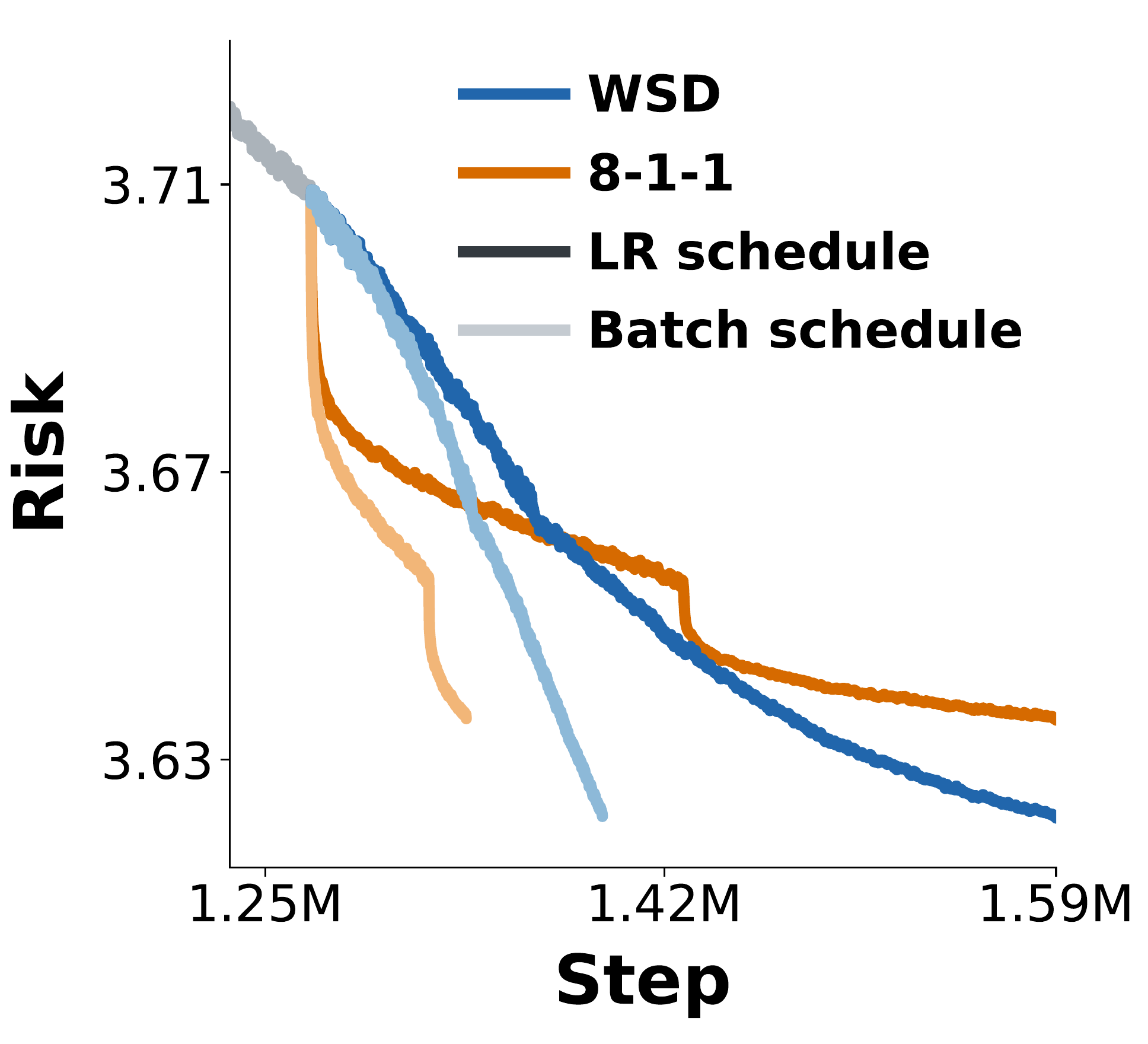
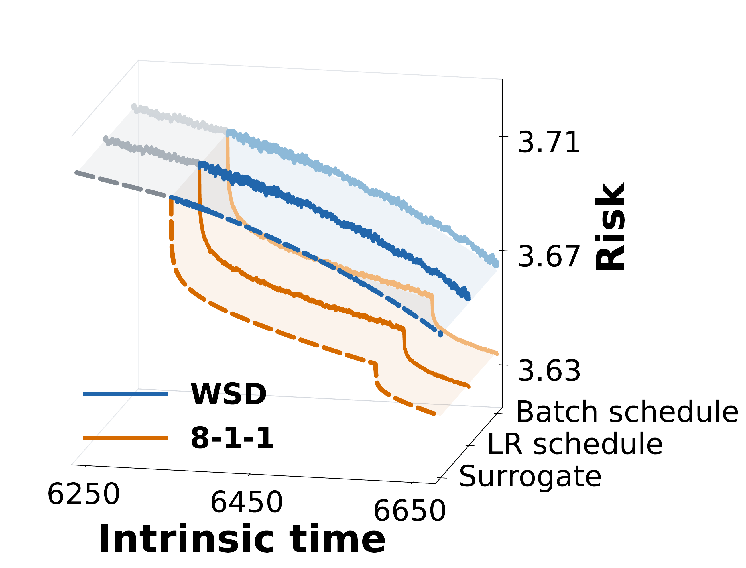
That is what we see. The paired curves separate against optimizer step, but nearly coincide against intrinsic time. Changing learning rate or batch size produces much the same loss response when the clock and ratio path are matched.
Fit one schedule and predict another
The paired runs share a ratio path. A harder test is to change it: can a response learned from the abrupt drops of 8-1-1 predict the gradual decline of WSD?
For LLM validation loss, we keep the forcing–memory structure but fit its component functions rather than use the random-feature model’s exact quantities. Building on Li et al.’s functional-scaling-law approach, we use the seven-parameter surrogate
\[\widehat L(T) =L_\infty+A_{\mathcal F}(1+T)^{-q_{\mathcal F}} +\int_0^T \frac{A_0+A_1(1+u)^{-q_{\mathcal F}}}{r(u)} \bigl(1+c_{\mathcal K}(T-u)\bigr)^{-q_{\mathcal K}} \,\mathrm du.\]The first two terms form a fitted baseline, not a separately measured noise-free trajectory. The integral models earlier noise weighted by what survives; its source amplitudes \(A_0,A_1\) are free parameters, not fixed by \(L_\infty\) and \(A_{\mathcal F}\). The parameters describe the effective response, while \(r(u)\) supplies the schedule.
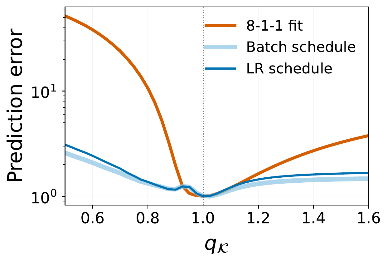
We fix \(q_{\mathcal K}=1\) and fit the other six parameters to raw validation loss from the fixed-batch 8-1-1 run. Then we freeze every parameter and replace only the ratio path with WSD’s. No WSD loss is used in this fit.
The predicted curve follows WSD’s measured validation loss, including its differently timed decline. It changes because the input schedule changes, not because we adjusted the response to fit another run.
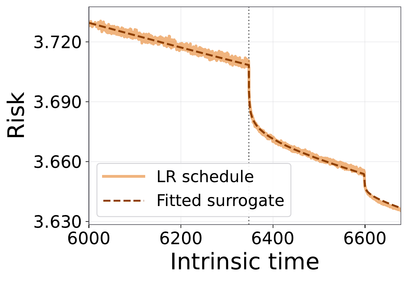
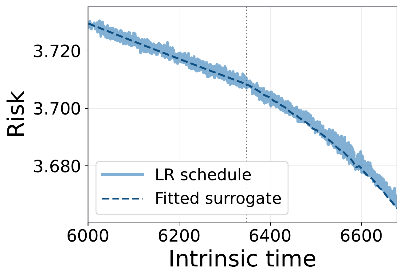
This is a more revealing test than fitting the two curves separately. A learning-curve model should earn our confidence by predicting what happens when training changes. Here the same response describes two different histories of noise injection.
Experiment and surrogate details
Training and matching. The preliminary 30M experiment continued one mature plain-SGD checkpoint under eleven ratio paths, all ending at the same intrinsic time. In the 300M comparison, each learning-rate/batch-size pair matches data, intrinsic-time increments, and \(B/\eta\) over groups of updates.
Surrogate parameters. The seven parameters are the floor \(L_\infty\), forcing amplitude \(A_{\mathcal F}\), source amplitudes \(A_0,A_1\), memory time-scale parameter \(c_{\mathcal K}\), and exponents \(q_{\mathcal F},q_{\mathcal K}\). The approximation separates the effective response as \(K(n,s)\approx J(T_s)k(T_n-T_s)\), where \(J\) is the source amplitude and \(k\) the propagation kernel.
With \(q_{\mathcal K}=1\), the other six parameters are fitted only to original, unsmoothed 8-1-1 measurements; no WSD loss enters that fit. The profile plot repeats this procedure for each fixed exponent and evaluates the resulting WSD prediction error.
Hybrid Muon. A short calibration selected a different clock and ratio for those runs: \(\widetilde T=\sum_t\eta_t^2\) and \(\widetilde r=B/\eta^2\). Those calibrated quantities brought its paired curves together as well.
Why does the memory exponent keep landing near one?
We fixed the memory exponent at one in that test. What happens if we let the fit choose it?
In separate fits, we let all seven parameters vary. Across different datasets and two model sizes, the memory exponent comes back close to one:
| Dataset and setting | \(q_{\mathcal K}\) | \(q_{\mathcal F}\) |
|---|---|---|
| OpenWebText, 124M, 2.5B tokens | 1.017 | 0.374 |
| FineWeb sample-10BT subset, 124M, 2.5B tokens | 0.952 | 0.405 |
| peS2o V2 s2orc full text, 124M, 2.5B tokens | 0.995 | 0.365 |
| OpenWebText, 300M, 6.5B tokens | 0.989 | 0.291 |
One lies at the LM/IM boundary: cumulative memory is finite on one side and keeps growing on the other, logarithmically at one. The fitted responses sit close to that boundary across these different tasks.
Do these tasks share an effective distribution of memory times? Or do finite training windows and trade-offs between fitted parameters pull the estimates toward the same value? The present curves do not distinguish those explanations. Changing the training horizon and measuring the response to deliberate perturbations would help tell them apart.
The larger lesson
A power-law curve can look deceptively complete: fit the slope, extrapolate, and the story seems finished. Yet the same shape can arise from learning remaining signal or from the persistence of earlier noise. Those explanations matter because they imply different responses when training changes.
That makes a schedule change more than a training choice. It is a way to ask what the curve has been hiding. If an explanation can follow the loss through that change without being fitted again, it tells us something that the original slope alone could not.
Further reading
- Empirical scaling laws: Kaplan et al. (2020), Scaling Laws for Neural Language Models. How language-model loss depends on model size, data, and compute.
- Spectral models: Paquette et al. (2024), 4+3 Phases of Compute-Optimal Neural Scaling Laws. A solvable model connecting data and target structure to compute-optimal regimes.
- Learning rate and batch size: Smith et al. (2018), Don’t Decay the Learning Rate, Increase the Batch Size. Experiments replacing learning-rate decay with batch-size growth.
- Predicting full trajectories: Li et al. (2025), Functional Scaling Laws in Kernel Regression: Loss Dynamics and Learning Rate Schedules. Intrinsic-time theory and surrogate prediction of LLM learning curves.
- Optimal schedules: Bordelon and Mori (2026), Theory of Optimal Learning Rate Schedules and Scaling Laws for a Random Feature Model. How optimal annealing depends on the spectrum and task.
This post is based on From Spectra to Joint Schedules in LLM Pre-training: 3+3(+2) Scaling-Law Regimes, joint work by Yichen Wang, Fanghui Liu, and Yudong Chen.